Introduction
In Python, modules and packages are essential for organizing and reusing code. As programs grow larger, splitting code into modules and packages makes it more maintainable, readable, and reusable.
- Module: A single Python file containing functions, classes, and variables.
- Package: A directory containing multiple modules and a special
__init__.pyfile (which can be empty).
Importing Modules and Packages
To use a module or package, you need to import it into your script. Python provides several ways to do this.
Basic Import
Use the import keyword followed by the module or package name.
Example: Importing numpy
| |
Importing Specific Modules or Functions
You can import specific modules or functions from a package using the from ... import ... syntax.
Example: Importing linalg from numpy
| |
Example: Importing a Specific Function
| |
Importing All Functions and Objects
You can import all functions and objects from a module using the * wildcard. However, this is not recommended as it can lead to namespace pollution and make the code harder to read.
Example: Importing Everything from numpy
| |
Renaming Modules on Import
You can assign an alias to a module when importing it using the as keyword. This is useful for shortening long module names.
Example: Importing numpy as np
| |
Namespaces in Python
A namespace is a container for identifiers (names of variables, functions, classes, etc.). It helps avoid naming conflicts by grouping related identifiers together.
- Module namespace: Each module has its own namespace.
- Global namespace: Contains all global variables and functions in a script.
- Local namespace: Contains variables and functions defined within a function.
Example: Accessing Functions from Different Namespaces
| |
The Python Standard Library
Python comes with a rich standard library containing over 200 modules for various tasks, such as:
- File I/O:
os,sys,pathlib - Data processing:
json,csv,pickle - Mathematics:
math,random,statistics - Networking:
http,urllib,socket - Concurrency:
threading,multiprocessing
Example: Using the math Module
| |
Creating Your Own Modules
You can create your own modules by writing Python code in a .py file and importing it into other scripts.
Example: Creating a Custom Module
- Create a file named
my_module.pywith the following content:
| |
- Import and use the module in another script:
| |
Creating Your Own Packages
To create a package:
- Create a directory with the name of your package.
- Add an empty
__init__.pyfile inside the directory (this file can also contain initialization code). - Add your modules (
.pyfiles) to the directory.
Example: Package Structure
my_package/
├── __init__.py
├── module1.py
└── module2.py
Example: Using a Custom Package
- Inside
module1.py:
| |
- Import and use the package in another script:
| |
Example: Scientific Computing with External Packages
Python has a vast ecosystem of third-party packages for scientific computing, data analysis, and visualization. Some popular ones include:
**numpy**: Numerical computing.**scipy**: Scientific computing.**matplotlib**: Data visualization.
Example: Projectile Motion Simulation
Here’s an example using numpy and matplotlib to simulate projectile motion with different friction models.
| |
Output:
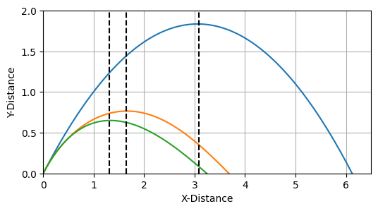
Projectile Motion
Installing Third-Party Packages
To use third-party packages, you need to install them first using a package manager like pip.
Example: Installing numpy and matplotlib
Run the following commands in your terminal:
| |
Best Practices for Using Modules and Packages
- Use Descriptive Names: Choose meaningful names for your modules and packages.
- **Avoid
from module import ***: It pollutes the namespace and makes the code harder to debug. - Use Aliases for Long Names: For example,
import numpy as np. - Organize Related Code: Group related functions and classes into modules and packages.
- Document Your Code: Use docstrings to explain the purpose of your modules and functions.
Conclusion
Modules and packages are powerful tools for organizing and reusing code in Python. They allow you to:
- Split large programs into manageable parts.
- Reuse code across multiple projects.
- Leverage the rich ecosystem of third-party packages.
By mastering modules and packages, you can write cleaner, more maintainable, and more efficient Python code.